TEMPORAL VORTEX MANUAL
WHAT IS SLITSCAN PHOTOGRAPHY?
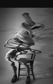
The origin of the term ‘slitscan’ comes from a photographic technique for capturing a span of time onto a single photographic Frame. (I’m using the word frame because we will be moving on over into video zones soon enough!) Typically one would expose a single frame instananeously to capture a still image. Slitscan photography however used a mechanical device over the lens to only allow a tiny ‘slit’ of light in at any given point and then the photographer would ‘scan’ the slit from right to left (or down to up) to allow different ‘slices’ of time light to expose the film at different physical locations. This is the important thing to remember about slitscan btw! There is a relationship between physical location on the frame and the relative location in TIME of what you can see on the frame!
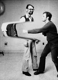
( Andrew Davidhazy {the person deftly avoiding the punch above) writes here about several important distinctions between various photographic techniques which can all have similar results as the slitscan process. I’m already digressionary and nitpicky enough about this kind of stuff so I don’t want to directly address these ideas here but I do want to make this information available for anyone interested in the practical mechanics of slitscan photography)
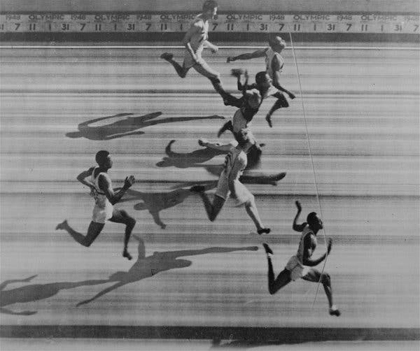
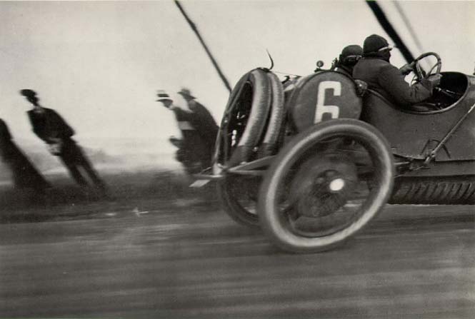
Uses for this photograph technique were not simply limited to surreal wiggly time worm humanoids! One of the primary commercial applications of this technique was for race tracks! Embedding multiple time slices from right to left on a photograph made it easier for folks to fdocument and prove which moving entity crossed the finish line first in neck and neck scenarios!
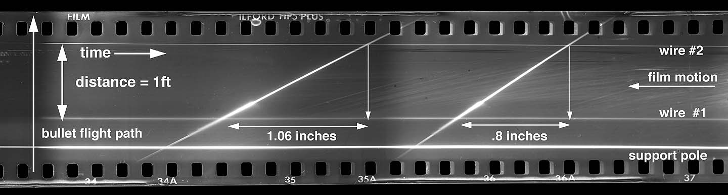
Industrial R&D found slitscan techniques to be useful for getting information on high speed ballistic events like missiles launching and bullets firing.
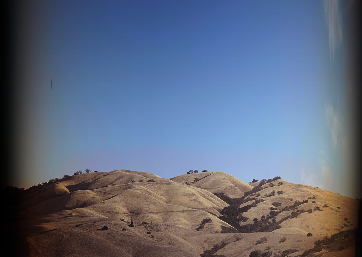
Creative usages included going in the opposite direction and slowing things down and rotating the camera as well for dizzying spacio-temporal panorama effects! With a low enough shutter speed one could capture night and day in the same photograh!
WHAT IS SLITSCAN ANIMATION AND WHAT IS SLITSCAN VIDEO?
As always, the obscenely profitable world of Hollywood Studio films encouraged folks to adapt any and all photographic techniques to video techniqes! (well yes, film at first, one can either think about ‘video’ as referring only to video taped things in the colloquial commercial sense or as ‘video’ simply referring to moving images in the colloquial signal oriented sense. I lean towards the second definition for convenience and will only talk specifically about film if theres something imperative about the film process that needs to be discussed)
Thus in order to shoot slitscan video in real time one has 2 options:
1. Figure out some way to store frames from the past and work out a way to use those past frames to create a new frame
2. Realize that its prior to 1980, theres not really such thing as a framebuffer in common usage yet, say fuck it and just use the same techniques from photography and simply generate a series of still images via slitscan which can then be animated more or less like stop motion animation!
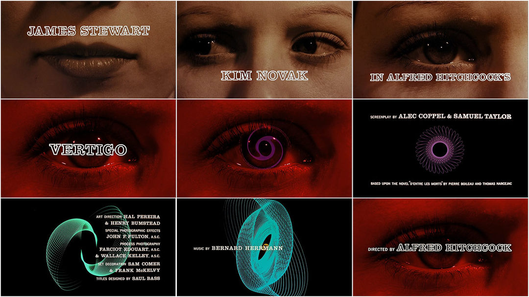
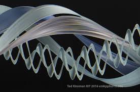
Needless to say, folks working in the 60s opted for number 2. The first use of slitscan techniques in cinema that I am aware of was by pioneering video and computer artist John Whitney’s hypnotizing spiral lissajous patterns generated for the title sequence of Hitchcock’s Vertigo.
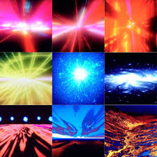
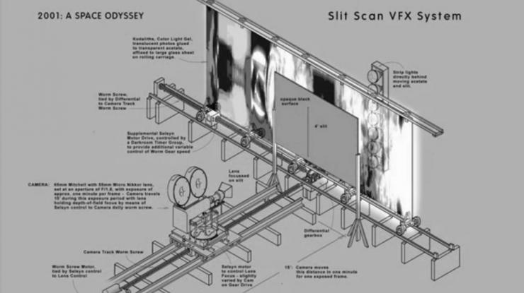
The famous cinematic dioramist Stanley Kubrick found out about the slitscan animation techinque via Whitney and had Douglass Trumbull build a massive rig and spend a couple of years putting together the ‘Star Gate’ sequence in 2001, frame by frame, using this crazy ass mechanical rig for zooming a camera while slitting the scan over and over and over again. Kubricks goal was to capture the theoretical experience of spatio temporal distortion as one reaches light speed, which in a very real way sums up the essense of what slitscan can do!
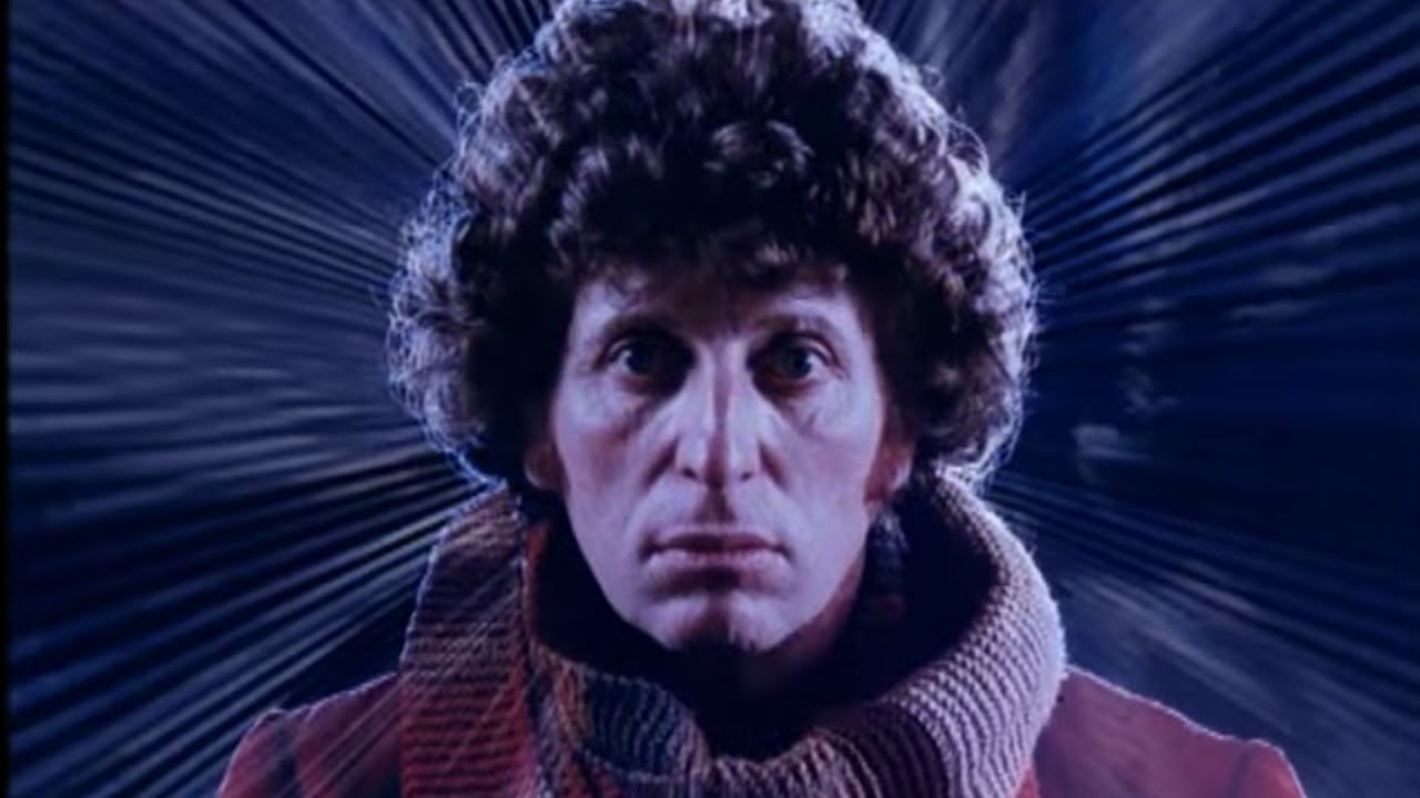
Of course after this movie came out, slitscan animation became the go to effect for sci fi ‘warp speed,’ ‘time travel,’ ‘look at these crazy blobs flying at yr face’ kind of texture for quite a while! Though like pretty much most of the use cases were just the exact same mechanical process as the 2001 sequence so nothing super crazy to note here, except for that it was the first time in history that camera feedback WASNT used for a Dr Who title sequence.
Artist and educator Golan Levin has put together a pretty remarkable list of slitscan examples from past to present over here along with a little Processing sketch for anyone interested in experimenting with slitscan photography in code zones!
One last video example that I can’t omit though is the amazing “The Fourth Dimension” by Zbigniew Rybczynski in 1988. What I find notable about this video compared to many other examples is the fact that in my experiences this is the most well executed example of slitscan Video techniques as opposed to Animation techniques.
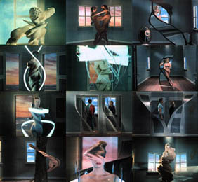
Instead of using animation techniques and ‘pre-processing’ they instead shot all the footage they wanted to use and then divided the individual frames into 480 vertical slices and reconstructed the video slice by slice in a meticulous, painstaking, and absurdly lengthy process! But as you can see, instead of just a bunch of flying blobs in hyperspace, this video features what seems like a surreal time bleeding as human figures noodle their way through 4 dimensional landscape! For me, this more than anything else inspired me to figure out how to get this happening as a real time effect.
MODERN SLITSCAN VIDEO TECHNIQUES
Ever since framebuffers and digital video processing techniqes became cheap and plentiful, doing full video slitscan as a post processing effect has become (relatively) commonplace. However the sheer scale of the temporal distortions involved made turning slitscan into a practical real time effect more than a little tricky! Other than the excellent SSSSCAN developed by Eric Souther and Jason Berngozzi as a part of the Signal Culture Apps collection and numerous one-off single purpose projects developed by individuals for artistic and/or commercial projects, there were not a lot of options out there for folks interested in doing realtime slitscan video. (ok yes theres that adobe thing in after effects, but like thats post processing only and also fuck adobe). Definitely head back up and check out that list by Golan for an incredibly diverse set of examples of adaptions of slitscan photography, animation, and video techniques! And so we move on to specifically talking about
TEMPORAL VORTEX
Let me first describe a bit of whats happening under the hood of this little beast before we talk about how to control it! First off TV (awkward nickname in this context, I know) saves the past 480 frames from input video in a buffer. Yes 480 frames! Given that TV also works at round about 20fps that means we’ve got 480/20 or round about 24 seconds of video being stored at any given point that we can access. For a bit of context Waaave Pool stores 60 frames or 2 seconds (WP is working with some different datatypes and can keep at a pretty solid 30fps) of past video. So 24 seconds is kind of massive!
Most digital approaches to this kind of system use fixed gradients for calculating what part of each frame gets pixels from what period of the past. This allows for higher resolutions, less memory impact, and potentially faster framerates but at a signficant cost of real time flexibility. My main goal with this (and every instrument I make) is to allow for the widest range of control and for the most amount of modulation possible without having the devices literally shorting out and melting.
Wait a second, I just mentioned gradients calculating time? What the fuck does that mean?? Ok, chill out, we are getting there! So for analog slitscan photography we could just scan around with the slit and analog natures of film take care of the rest. In digital slitscan video theres no physical scan, theres no physical slit, we can theoretically just get pixel data for anywhere in the frame from anywhere in that 480 frame buffer! But still its pretty helpful to think about how we can abstract this process for performance!
A fairly standard approach for understanding digital slitscan photography is the concept of using a greyscale gradient as a map or mask for calculating what part of each frame gets mapped to what time. For example in the picture above lets say that a completely black pixel maps to 0 frames back while a completely white pixel maps to 480 frames back. Thus from left to right we would have a temporal gradient from the very very recent past to all the way back 480 frames in the past!
My feelings on fixed gradients as maps tho were that it did not really translate into being a fully developed instruments. Playing around with fixed gradients systems felt like having a very nice instagram filter but it was pretty easy to get bored after not very much time at all. Thus I decided to toss out the fixed gradient idea and instead use a system of 2 video oscillators to generate dynamic gradients to use for maps! At that point TV went from being a sketch of an idea to pretty much a full fledged instrument!
Video Oscillators
So lets talk about the oscillators for a bit! If you are unclear on the concept of Video Oscillator and what makes it different from an Audio Oscillator I’d recommend checking out my Spectral Mesh and/or Artifical Life manuals for a more detailed explanation! Short answer is that video has one more dimension than audio so video oscs have 3 arguments: amplitude, rate, and frequency. Amplitude maps to brightness (amp=0 -> black, amp=1 -> white), rate is the change between seperate frames, and frequency is how many oscillations happen per frame!
Each Oscillator has control for each of the above listed parameters as well as an additional argument I call ‘angle’ which controls what direction the oscillators oscillate in!
The default waveshape for each oscillator is Triangle (I tried sine at first but the nonlinear amplitude curve resulted in less pleasing temporal gradients) with options to switch to Sawtooth, Square, or Perlin Noise.
The default angle for each oscillator is horizontal and vertical respectively. One can also switch from either of those modes and make the oscillators Radial instead. Radial means that instead of going right to left, up to down, or anything in between, the oscillator radiates outward from the center for the screen! The different radial options are Circular, 4 Quadrant Parabolic, and like Cubic? Note that radial shapes bypass angular controls, and that Perlin Noise bypasses radial oscillators!
COMBINING OSCILLATORS
The oscillators can be mixed together in a various ways. The default method is just summing and clamping the combined outputs together, this requires a bit of gain staging on each individual osc amplitude to make it work (i.e if both oscillators are at max amp then yr more or less just going to have a clamped whiteout happening without much gradient) but still quite useful in a lot of situations
Wrap Mode adds the two oscillators together and wraps the signal over 1 through 0. Lots of discontinuities happening here!
Foldover adds the two oscillators together and folds the signal back over from 1, so if osc1 at .75 and osc2 at .5 at a given pixel the output will be .75. Foldover means less discontinuities overall unless you have a Square wave involved!
Ringmod & fold mode multiplies the two oscillators together and then does foldover on everything over 1. Note that if either oscillator is at 0 then the output will always be 0.
Shaper & fold mode remaps the output of each osc from 0 to 2PI, sums them together, uses the summed output as an argument in a sine function and then folds everything over 1 or under 0 back into the 0-1 range
Cross Mod Shaper & fold mode uses the output from each indivual oscillator to recalculate each individual oscillator with phase mod, sums them together, and folds over 1 and under 0. Yes that is a mouthful. Let me just share the code and walk through things here
Create a dummy variable to hold the original output from osc0
Replace osc0 output with a new oscillating value calculated by adding the original argument of osc0 with the output from osc1.
Do the same with Osc1 but use the dummy variable of the original output of osc0.
| “float osc0_displace_dummy=osc0_displace;” |
| “osc0_displace=d_osc0_amp*time_osc(osc0_argument+6.18*osc1_displace,osc0_shape,0,i,j);” |
| “osc1_displace=d_osc1_amp*time_osc(osc1_argument+6.18*osc0_displace_dummy,osc1_shape,1,i,j);” |
| “displacement_amount_normalized=(osc0_displace+osc1_displace)/2.0f;” |
Yeah maybe that doesn’t help most folks. You can just think Cross mod and think about how that incredibly vague parameter used to exist on analog synths all over the place back in the day without any kinds of details on whether it was ring mod, phase mod, linear fm, exponential fm, hard sync etc etc.
RGB displacement
But wait thats not all. A pretty quirky addition to TV is the ability to set temporal offsets for the individual RGB channels of the video! RGB means Red Green Blue and refers to the default color space of this (and actually all of) my instruments. The offsets are calculated by taking the output from the combined oscilators and then adding a linear offset for each of the color channels based on how far you’ve twisted the knobs/sliders! To isolate and get a good feel for this effect try feeding TV a signal thats just a white moving shape on a black background, set up a simple displacement with 1 oscillator and then experiment with offsetting first R G and B individually and then all together!
Blurring
Something to note about the internal processing of TV, all video inputs get downsampled to 320x240 and color information for each pixel gets downsampled into 7 bits per each RGB channel. This is pretty much the smallest I could make each Frame live as a datatype without getting too grunchy and choppy. Nevertheless it is possible that the output from TV can get a little chunky and discrete at times, thus I tossed in a little blur function at the end of the chain to smooth things out!
Looping
Temporal Resolution
Video Oscillator Terminology
RATE means the change between frames
FREQUENCY means the amount of oscillations within any single frame
AMP means brightness with 0 being completely black and 1 being completely white
1.5 updates
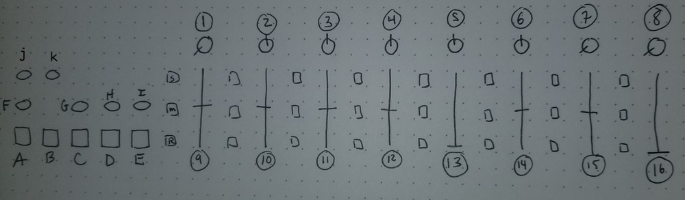
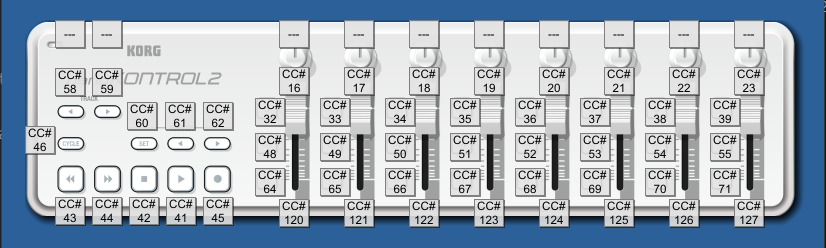
The only real change is that midi latching has been implemented. this means that whenver you boot up or whenever you reset the controls, when you move a slider or knob it won’t change the value you see on the output until you move through the default starting point. only 1, 2 and 9 have default values that aren’t zero so experiment with these a bit on yr own to get a handle on things at first!
1. Time_Osc0 Rate
2. Time_Osc0 Frequency
9. Time_Osc0 Amplitude
10. Time_Osc0 Angle
Time_Osc0 Wave Shapes
default is Triangle
S9. Sawtooth
M9. Square
R9. Perlin Noise
Time_Osc0 Radial Forms
S10. Circle
S10. Parabolic
S10. Vulvic?
Radial forms can be affected by all waveshapes except for Perlin Noise. For example pressing M9 and S11 will result in radial hard edge circle shapes. Pressing R9 and S11 will just result in Perlin Noise though.
3. Time_Osc1 Rate
4. Time_Osc1 Frequency
11. Time_Osc1 Amplitude
12. Time_Osc1 Angle
Time_Osc1 Wave Shapes
default is Triangle
S11. Sawtooth
M11. Square
R11. Perlin Noise
Time_Osc1 Radial Forms
S12. Circle
M12. Parabolic
S12. Vulvic?
RGB
5. Red Offset
6. Green Offset
14. Blue Offset
13. Blur
7. Loop Point Begin
15. Loop Point End
8. Temporal Resolution
Osc Combinations
These are all various ways of mixing together the dual oscillators. default is sum and clamp, meaning its pretty easy to just have everything clamped at full brightness nearly constantly
A. wrap mode
B. foldover
C. ringmod and fold
D. shaper and fold
E. cross mod shaper and fold
picture from chrono cross
good bye

If you appreciate the public domain open source software and educational materials I provide and can afford to spare some cash it is highly appreciated! The more donations I recieve the more time I have to spend on developing these resources! Please also consider subscribing to my patreon page as small amounts of regular income are appreciated as well! Or you could also support my ko-fi if you like getting stickers and stuff on a regular basis.